library(tidyverse)
library(skimr)Example EDA
Basic steps taken in this rough exploration of data….
- import data
- wrangle data
- join data
- visualize data
A brief discussion of packages which proport to perform EDA for you can be found in the Get Started section of this site.
Note: This page is not intended to teach formal EDA. What happens on this page is merely a brutal re-enactment of some informal explorations that a person might take as they familiarize themselves with new data. If you’re like most people, you might want to skip to the visualizations. Meanwhile, the sections and code-chunks preceding visualization are worth a glance.

Import data
The data come from a TidyTuesday, a weekly social learning project dedicated to gaining practical experience with R and data science. In this case the TidyTuesday data are based on International Trail Running Association (ITRA) data but inspired by Benjamin Nowak, . We will use the TidyTuesday data that are on GitHub. Nowak’s data are also available on GitHub.
race_df <- read_csv("https://raw.githubusercontent.com/rfordatascience/tidytuesday/master/data/2021/2021-10-26/race.csv")
rank_df <- read_csv("https://raw.githubusercontent.com/rfordatascience/tidytuesday/master/data/2021/2021-10-26/ultra_rankings.csv")glimpse(race_df)Rows: 1,207
Columns: 13
$ race_year_id <dbl> 68140, 72496, 69855, 67856, 70469, 66887, 67851, 68241,…
$ event <chr> "Peak District Ultras", "UTMB®", "Grand Raid des Pyréné…
$ race <chr> "Millstone 100", "UTMB®", "Ultra Tour 160", "PERSENK UL…
$ city <chr> "Castleton", "Chamonix", "vielle-Aure", "Asenovgrad", "…
$ country <chr> "United Kingdom", "France", "France", "Bulgaria", "Turk…
$ date <date> 2021-09-03, 2021-08-27, 2021-08-20, 2021-08-20, 2021-0…
$ start_time <time> 19:00:00, 17:00:00, 05:00:00, 18:00:00, 18:00:00, 17:0…
$ participation <chr> "solo", "Solo", "solo", "solo", "solo", "solo", "solo",…
$ distance <dbl> 166.9, 170.7, 167.0, 164.0, 159.9, 159.9, 163.8, 163.9,…
$ elevation_gain <dbl> 4520, 9930, 9980, 7490, 100, 9850, 5460, 4630, 6410, 31…
$ elevation_loss <dbl> -4520, -9930, -9980, -7500, -100, -9850, -5460, -4660, …
$ aid_stations <dbl> 10, 11, 13, 13, 12, 15, 5, 8, 13, 23, 13, 5, 12, 15, 0,…
$ participants <dbl> 150, 2300, 600, 150, 0, 300, 0, 200, 120, 100, 300, 50,…glimpse(rank_df)Rows: 137,803
Columns: 8
$ race_year_id <dbl> 68140, 68140, 68140, 68140, 68140, 68140, 68140, 68140…
$ rank <dbl> 1, 2, 3, 4, 5, 6, 7, 8, 9, 10, 11, 12, 13, NA, NA, NA,…
$ runner <chr> "VERHEUL Jasper", "MOULDING JON", "RICHARDSON Phill", …
$ time <chr> "26H 35M 25S", "27H 0M 29S", "28H 49M 7S", "30H 53M 37…
$ age <dbl> 30, 43, 38, 55, 48, 31, 55, 40, 47, 29, 48, 47, 52, 49…
$ gender <chr> "M", "M", "M", "W", "W", "M", "W", "W", "M", "M", "M",…
$ nationality <chr> "GBR", "GBR", "GBR", "GBR", "GBR", "GBR", "GBR", "GBR"…
$ time_in_seconds <dbl> 95725, 97229, 103747, 111217, 117981, 118000, 120601, …EDA with skimr
skim(race_df)| Name | race_df |
| Number of rows | 1207 |
| Number of columns | 13 |
| _______________________ | |
| Column type frequency: | |
| character | 5 |
| Date | 1 |
| difftime | 1 |
| numeric | 6 |
| ________________________ | |
| Group variables | None |
Variable type: character
| skim_variable | n_missing | complete_rate | min | max | empty | n_unique | whitespace |
|---|---|---|---|---|---|---|---|
| event | 0 | 1.00 | 4 | 57 | 0 | 435 | 0 |
| race | 0 | 1.00 | 3 | 63 | 0 | 371 | 0 |
| city | 172 | 0.86 | 2 | 30 | 0 | 308 | 0 |
| country | 4 | 1.00 | 4 | 17 | 0 | 60 | 0 |
| participation | 0 | 1.00 | 4 | 5 | 0 | 4 | 0 |
Variable type: Date
| skim_variable | n_missing | complete_rate | min | max | median | n_unique |
|---|---|---|---|---|---|---|
| date | 0 | 1 | 2012-01-14 | 2021-09-03 | 2017-09-30 | 711 |
Variable type: difftime
| skim_variable | n_missing | complete_rate | min | max | median | n_unique |
|---|---|---|---|---|---|---|
| start_time | 0 | 1 | 0 secs | 82800 secs | 05:00:00 | 39 |
Variable type: numeric
| skim_variable | n_missing | complete_rate | mean | sd | p0 | p25 | p50 | p75 | p100 | hist |
|---|---|---|---|---|---|---|---|---|---|---|
| race_year_id | 0 | 1 | 27889.65 | 20689.90 | 2320 | 9813.5 | 23565.0 | 42686.00 | 72496.0 | ▇▃▃▂▂ |
| distance | 0 | 1 | 152.62 | 39.88 | 0 | 160.1 | 161.5 | 165.15 | 179.1 | ▁▁▁▁▇ |
| elevation_gain | 0 | 1 | 5294.79 | 2872.29 | 0 | 3210.0 | 5420.0 | 7145.00 | 14430.0 | ▅▇▇▂▁ |
| elevation_loss | 0 | 1 | -5317.01 | 2899.12 | -14440 | -7206.5 | -5420.0 | -3220.00 | 0.0 | ▁▂▇▇▅ |
| aid_stations | 0 | 1 | 8.63 | 7.63 | 0 | 0.0 | 9.0 | 14.00 | 56.0 | ▇▆▁▁▁ |
| participants | 0 | 1 | 120.49 | 281.83 | 0 | 0.0 | 21.0 | 150.00 | 2900.0 | ▇▁▁▁▁ |
Read more about automagic EAD packages.
Freewheelin’ EDA
race_df |>
  count(country, sort = TRUE) |>
  filter(str_detect(country, regex("Ke", ignore_case = TRUE)))
race_df |>
filter(country == "Turkey")race_df |>
count(participation, sort = TRUE)race_df |>
count(participants, sort = TRUE)skim(rank_df)| Name | rank_df |
| Number of rows | 137803 |
| Number of columns | 8 |
| _______________________ | |
| Column type frequency: | |
| character | 4 |
| numeric | 4 |
| ________________________ | |
| Group variables | None |
Variable type: character
| skim_variable | n_missing | complete_rate | min | max | empty | n_unique | whitespace |
|---|---|---|---|---|---|---|---|
| runner | 0 | 1.00 | 3 | 52 | 0 | 73629 | 0 |
| time | 17791 | 0.87 | 8 | 11 | 0 | 72840 | 0 |
| gender | 30 | 1.00 | 1 | 1 | 0 | 2 | 0 |
| nationality | 0 | 1.00 | 3 | 3 | 0 | 133 | 0 |
Variable type: numeric
| skim_variable | n_missing | complete_rate | mean | sd | p0 | p25 | p50 | p75 | p100 | hist |
|---|---|---|---|---|---|---|---|---|---|---|
| race_year_id | 0 | 1.00 | 26678.70 | 20156.18 | 2320 | 8670 | 21795 | 40621 | 72496 | ▇▃▃▂▂ |
| rank | 17791 | 0.87 | 253.56 | 390.80 | 1 | 31 | 87 | 235 | 1962 | ▇▁▁▁▁ |
| age | 0 | 1.00 | 46.25 | 10.11 | 0 | 40 | 46 | 53 | 133 | ▁▇▂▁▁ |
| time_in_seconds | 17791 | 0.87 | 122358.26 | 37234.38 | 3600 | 96566 | 114167 | 148020 | 296806 | ▁▇▆▁▁ |
rank_df |>
  filter(str_detect(nationality, regex("ken", ignore_case = TRUE)))
rank_df |>
arrange(rank)rank_df |>
count(rank, sort = TRUE)rank_df |>
drop_na(rank) |>
count(rank, gender, age, sort = TRUE)race_df |>
count(distance, sort = TRUE)rank_df |>
filter(race_year_id == 41449)race_df |>
filter(race_year_id == 41449)race_df |>
filter(distance == 161)race_dfrace_df |>
count(race, city, sort = TRUE)race_df |>
filter(race == "Centurion North Downs Way 100")race_df |>
filter(race_year_id == 68140)race_df |>
filter(race == "Millstone 100")race_df |>
filter(event == "Peak District Ultras")race_df |>
count(race, sort = TRUE) race_df |>
count(city, sort = TRUE) race_df |>
count(event, sort = TRUE) race_df |>
filter(event == "Burning River Endurance Run")Visualize, wrangle, and summarize
Here I’m using this State of Ultra Running report as a model to demonstrate some of the capabilities of R / Tidyverse
join datasets
Join, Assign, and Pipe
In this case I want to join the two data frames rank_df and race_df using the left_join() function.
I can assign the output of a “data pipe” (i.e. data sentence) to use in subsequent code-chunks. A common R / Tidyverse assignment operator is the <- characters. You can read this as “gets value from”.
Additionally, I’m using a pipe operator (|>) as a conjunction to connect functions. In this way I can form a data sentence. Many people call the data sentence a data pipe, or just a pipe. You may see another common pipe operator: %>%. \> and %>% are synonymous.
using dplyr::left_join() I combine the two data sets and then use {ggplot2} to create a line graph of participants by year.
my_df_joined <- rank_df |>
  left_join(race_df, by = "race_year_id") |>
  mutate(my_year = lubridate::year(date))
Viz participants
Let’ make a quick line plot showing how many people participate in races each year. Here we have a date field this is also a date data-type. Data types are important and in this example using a data data-type means {ggplot2} will simplify our x-axis labels.
Here we use the {lubridate} package to help manage my date data-types. We also use {ggplot2} to generate a line graph as a time series via the {ggplot2} package and a geom_line() layer. Note that {ggplot2} uses the ‘+’ as the conjunction or pipe.
rank_df |>
  left_join(race_df |> select(race_year_id, date), by = "race_year_id") |>
  mutate(my_year = lubridate::year(date)) |>
  count(my_year, sort = TRUE) |>
  ggplot(aes(my_year, n)) +
  geom_line()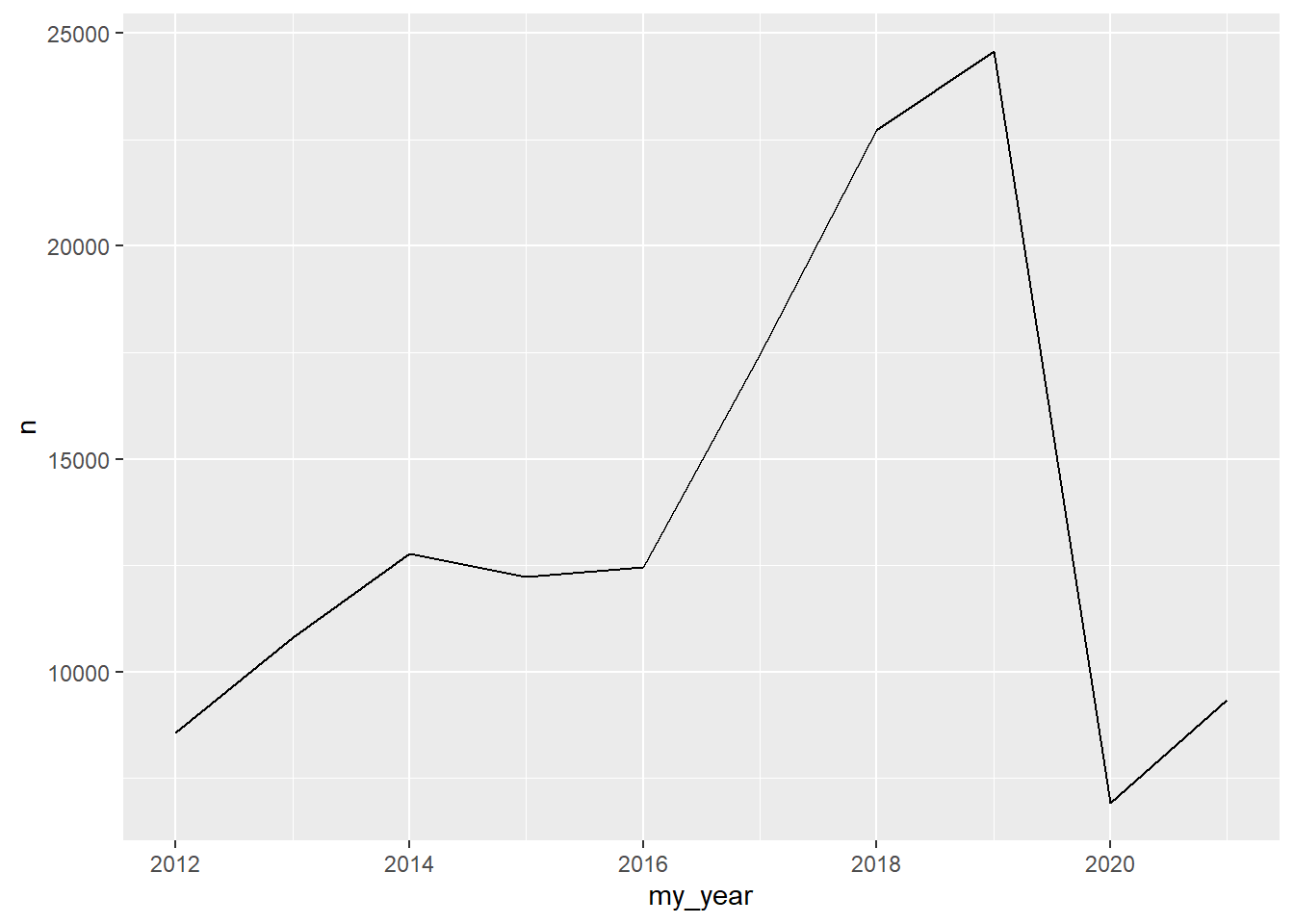
by distance
Here I use count() in different ways to see what I can see. I comment out each attempt before settling on summarizing a table of total country participants by year.
my_df_joined |>
  mutate(participation = str_to_lower(participation)) |>
  # count(participation, sort = TRUE)
  # count(city) |>
  # count(race) |>
  count(my_year, country, sort = TRUE)
my_df_joined |>
mutate(participation = str_to_lower(participation)) |>
count(my_year, country, sort = TRUE) |>
drop_na(country) |>
mutate(country = fct_lump_prop(country, prop = .03)) |>
ggplot(aes(my_year, n)) +
geom_line(aes(color = country))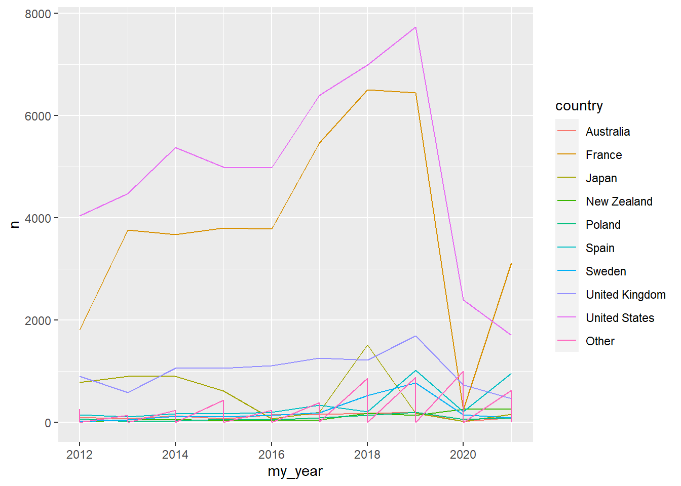
by country
I used fct_lump_prop() in the previous code-chunk to lump the country variable into categories by frequency. Here we refine the categories into specific levels. We are still mutating the country variable as a categorical factor; this time using the fct_other() function of {forcats} with some pre-defined levels (see the my_levels vector in the code-chunk below).
my_levels <- c("United States", "France", "United Kingdom", "Spain")

my_df_joined |>
  mutate(country = fct_other(country, keep = my_levels)) |>
  count(my_year, country, sort = TRUE) |>
  drop_na(country) |>
  ggplot(aes(my_year, n, color = country)) +
  geom_line() +
  geom_point() +
scale_color_brewer(palette = "Dark2") 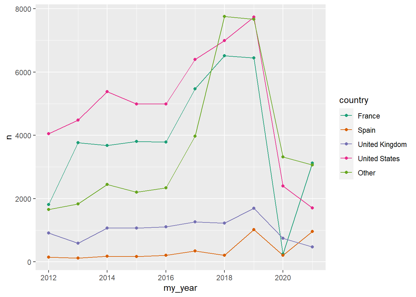
Country race-host
my_df_joined |>
  drop_na(country) |>
  mutate(country = fct_lump_n(country, n = 7)) |>
  count(country, sort = TRUE) |>
  ggplot(aes(x = n, y = fct_reorder(country, n))) +
  geom_col()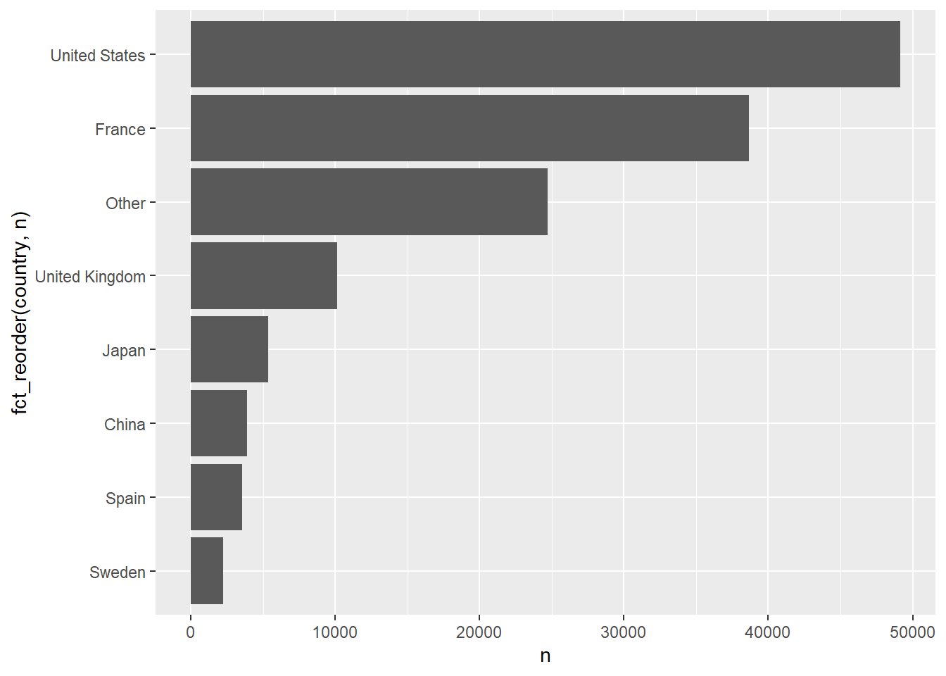
Nationality of runner
my_df_joined |>
  mutate(nationality = fct_lump_n(nationality, n = 7)) |>
  count(nationality, sort = TRUE) |>
  ggplot(aes(n, fct_reorder(nationality, n))) +
  geom_col()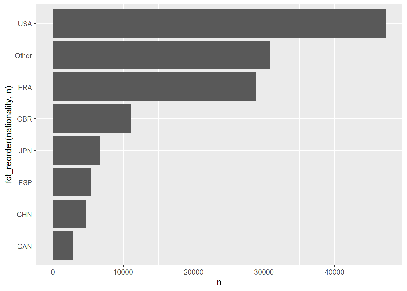
Unique participants
my_df_joined |>
  distinct(my_year, runner) |>
  count(my_year) |>
  ggplot(aes(my_year, n)) +
  geom_line()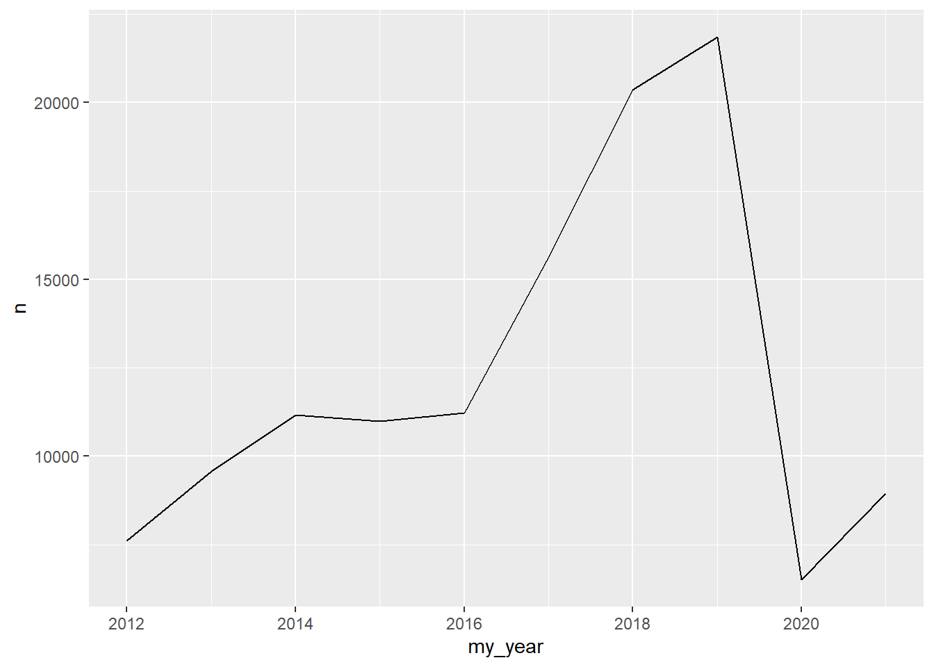
Participant frequency separated by gender
Note the use of count, if_else, as.character, and group_by to transform the data for visualizing. Meanwhile, the visual bar graph is a proportional graph with the y-axis label by percentage. We do this by manipulating the plot scales. Scales are also used to choose colors from a predefined palette (i.e. “Dark2”.) Findally, we facet the plot by gender (See facet_wrap()).
my_df_joined |>
  count(my_year, gender, runner, sort = TRUE) |>
  mutate(n_category = if_else(n >= 5, "more", as.character(n))) |>
  group_by(my_year) |>
  mutate(total_races = sum(n)) |>
  ungroup() |>
  ggplot(aes(my_year, total_races))  +
  geom_col(aes(fill = fct_rev(n_category)), position = "fill") +
  scale_fill_brewer(palette = "Dark2") +
  scale_y_continuous(labels = scales::percent) +
facet_wrap(vars(gender)) 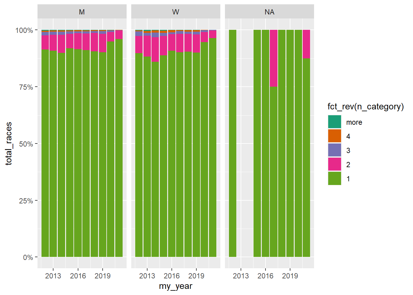
Pace per mile
We want to calculate a value for each runner’s pace (i.e. minute_miles). We have to create and convert a character data-type of the time variable into a numeric floating point (or dbl) data-type so that we can calculate pace (i.e. race-minutes divided by distance.) These data transformations required a lot of manipulation as I was thinking through my goal. I could optimized this code, perhaps. However it works and I’ve got other things to do. Do I care if the CPU works extra hard? No, not in this case.
my_df_joined |>
  mutate(time_hms = str_remove_all(time, "[HMS]"), .after = time) |>
  mutate(time_hms = str_replace_all(time_hms, "\\s", ":")) |>
  separate(time_hms, into = c("h", "m", "s"), sep = ":") |>
  mutate(bigminutes = (
    (as.numeric(h) * 60) + as.numeric(m) + (as.numeric(s) * .75)
    ), .before = h) |>
  mutate(pace = bigminutes / distance, .before = bigminutes) |>
  drop_na(pace, distance, my_year) |>
  filter(distance > 0,
         pace > 0) |>
  group_by(my_year, gender) |>
  summarise(avg_pace = mean(pace), max_pace = max(pace), min_pace = min(pace)) |>
  pivot_longer(-c(my_year, gender), names_to = "pace_type")  |>
  separate(value, into = c("m", "s"), remove = FALSE) |>
  mutate(h = "00", .before = m) |>
  mutate(m = str_pad(as.numeric(m), width = 2, pad = "0")) |>
  mutate(s = str_pad(round(as.numeric(str_c("0.",s)) * 60), width = 2, pad = "0")) |>
  unite(minute_miles, h:s, sep = ":") |>
  mutate(minute_miles = hms::as_hms(minute_miles)) |>
  # drop_na(gender) |>
  ggplot(aes(my_year, minute_miles)) +
  geom_line(aes(color = pace_type), size = 1) +
  scale_color_brewer(palette = "Dark2") +
  theme_classic() +
  facet_wrap(vars(gender))
`summarise()` has grouped output by 'my_year'. You can override using the
`.groups` argument.Warning: Using `size` aesthetic for lines was deprecated in ggplot2 3.4.0.
ℹ Please use `linewidth` instead.
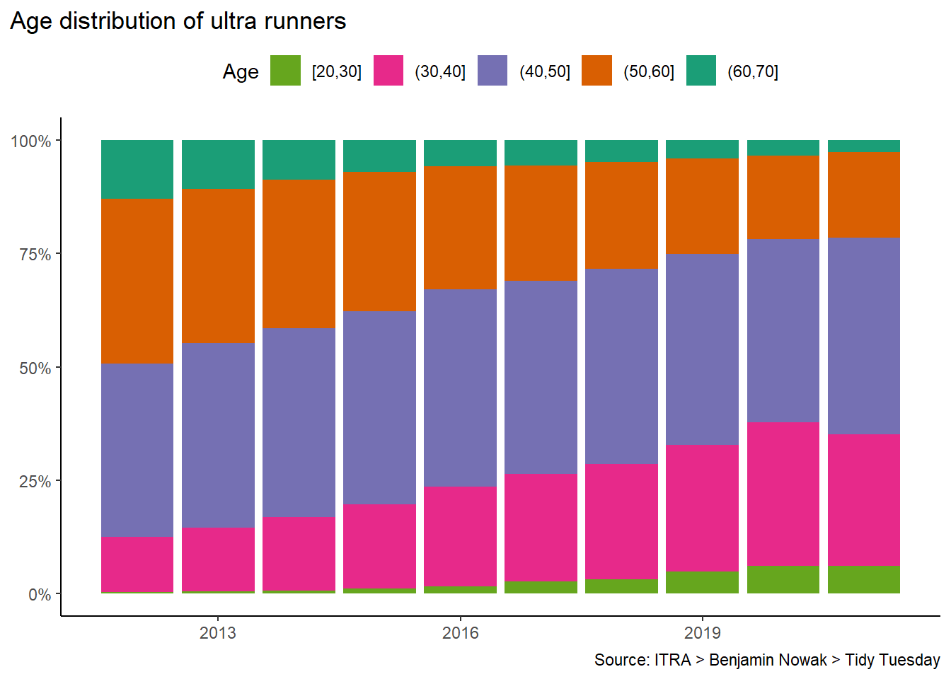
Age trends
In this code-chunk we use a {ggplot2} function, cut_width(), to generate rough categories by age. dplyr::case_when() is a more thorough and sophisticated way to make some cuts in my data, but ggplot2::cut_width() works well for a quick visualization.
Note the use of labels, scales, themes, and guides in the last visualization. A good plot will need refinement with some or all of these functions.
my_df_joined |>
  mutate(age_cut = cut_width(age, width = 10, boundary = 0), .after = age) |>
  count(age_cut, gender, sort = TRUE)
my_df_joined |>
filter(age < 80) |>
drop_na(gender) |>
ggplot(aes(y = cut_width(age, width = 10, boundary = 0))) +
geom_bar(aes(fill = gender)) +
facet_wrap(vars(gender))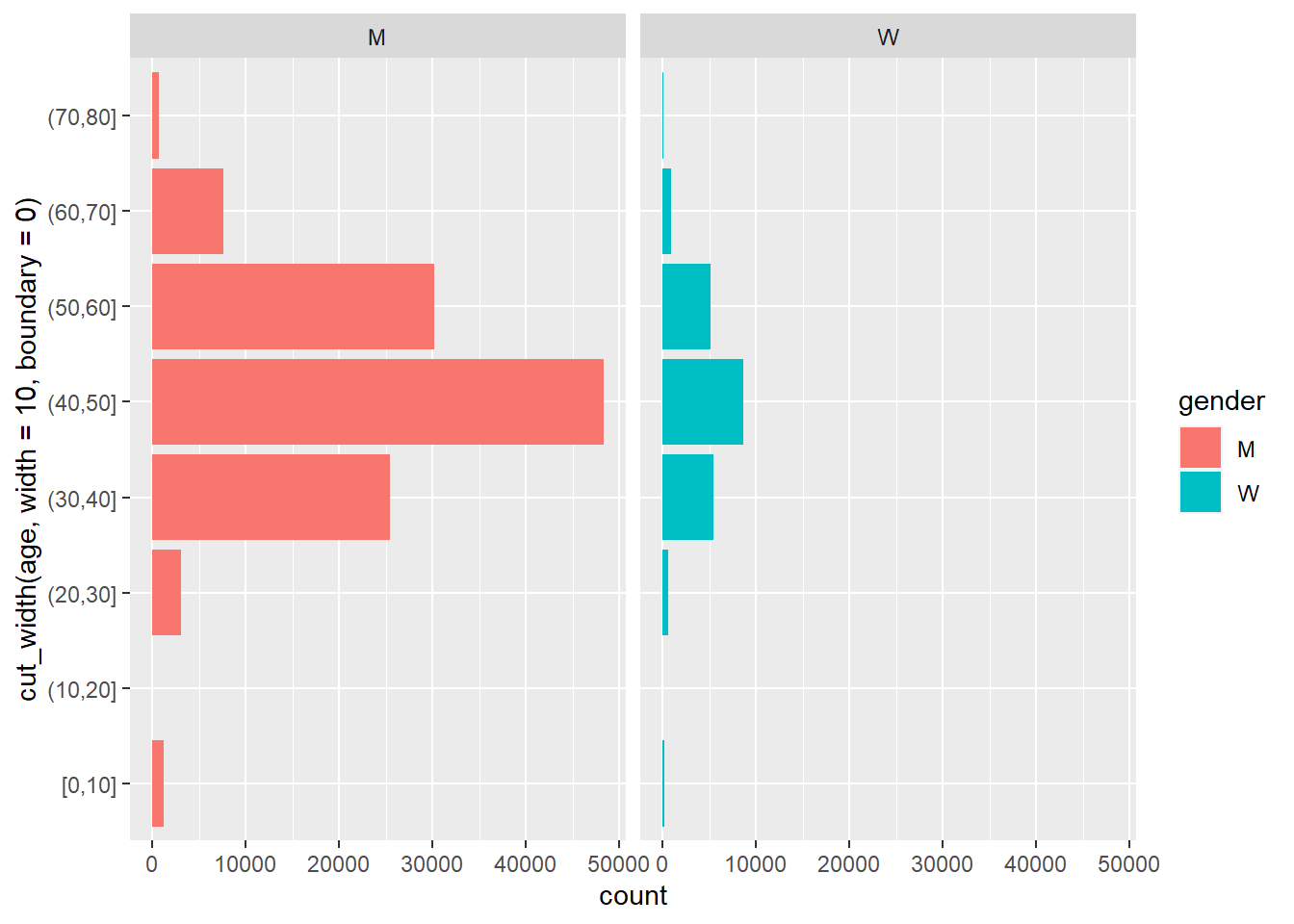
my_df_joined |>
  filter(age < 70, age >= 20) |>
  drop_na(gender) |>
  ggplot(aes(my_year)) +
  geom_bar(aes(fill = fct_rev(cut_width(age, width = 10, boundary = 0))), position = "fill") +
  scale_y_continuous(labels = scales::percent) +
  scale_fill_brewer(palette = "Dark2") +
  labs(fill = "Age", title = "Age distribution of ultra runners",
       caption = "Source: ITRA > Benjamin Nowak > Tidy Tuesday",
       x = NULL, y = NULL) +
  theme_classic() +
  theme(legend.position = "top", plot.title.position = "plot") +
  guides(fill = guide_legend(reverse = TRUE))