Pivot

Often our goal is to reshape a data frame into a tidy data (Wickham 2014) format. This is also known as tall data or long data. The {tidyr} package has functions to reshape data into tall or wide formats. When coding in the tidyverse context, tall data is much easier to iterate over — without ever writing for loops or other kind of flow control. Later, in the advance section, we’ll introduce the {purrr} package for more powerful iteration.

Image credit: Tidy data from the book _R for Data Science_

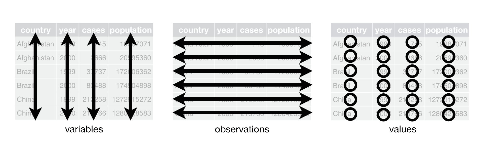
Tidy data¹

• Every variable is a column
• Every row is an observation
• Every cell is a single value

Many of the {dplyr} functions help with making data tidy. Additionally, in this chapter, we focus on using the {tidyr} function: pivot_longer, as well as pivot_wider.

See Also the Pivot Vignette

Load library packages

Load the {tidyverse} meta package which loads eight packges, including {tidyr}.

library(tidyverse)

Data

Our practice datasets are now available.

data(relig_income)
data(fish_encounters)

Longer

pivot_longer()

We can start with the tidyr::relig_income data frame. This is wide data and does not conform to tidy data (Wickham 2014) principles. This makes it harder to iterate by row because there are multiple observations in each row. In this data frame, each row has 10 observations, one observation for each income category.

relig_income

We can pivot this to tall data (i.e. pivot_longer) so that we have one observation per row for a total of 180 rows.

relig_income %>%
  pivot_longer(-religion, names_to = "income", values_to = "count")

Wider

Of course, sometimes we want wide data. There are a variety of reasons to wrangle data into a wide-data format. We use pivot_wider to accomplish this.

fish_encounters

fish_encounters %>% 
  pivot_wider(names_from = station, values_from = seen)

Why pivot data?

Why pivot data? Your analysis may require the shape of data to match a particular structure. For example, ggplot generally prefers long tidy data. Once the data are properly shaped, analysis and variations becomes easier. Below is a quick example of using ggplot to format data in a long and tidy shape to create a bar plot. Of course, the plot needs some refining. Hence, improvements become easier to accomplish with the tall data shape. Nonetheless, below shows an initial draft of a bar plot.

relig_income %>%
  pivot_longer(-religion, names_to = "income", values_to = "count") %>% 
  ggplot(aes(religion, count, fill = income)) +
  geom_col()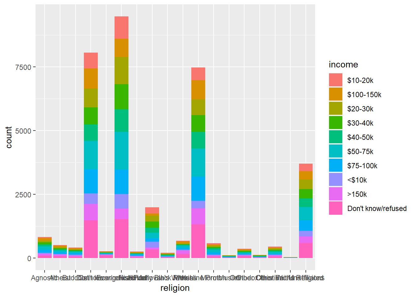

Once the data are properly shaped, variations on analysis becomes easier. Next, I format some variables as categorical vectors (i.e. factors), so that I can redraw the plot for clarity.

My goal is to format the vectors as factors using the forcats package. This will allow me to arrange

• the order of the bars
• the order of the stacked elements of each bar
• the order of the Legend

I will also change the color scheme of the discrete color from the fill argument, in combination with the scale_fill_viridis_d function.

inc_levels = c("Don't know/refused",
               "<$10k", "$10-20k", "$20-30k", "$30-40k",
               "$40-50k", "$50-75k", "$75-100k", "$100-150k",
               ">150k")

relig_income %>%
  pivot_longer(-religion, names_to = "income", values_to = "count") %>% 
  mutate(income = fct_relevel(income, inc_levels)) %>% 
  ggplot(aes(fct_reorder(religion, count), 
             count, fill = fct_rev(income))) +
  geom_col() +
  scale_fill_viridis_d(direction = -1) +
  coord_flip()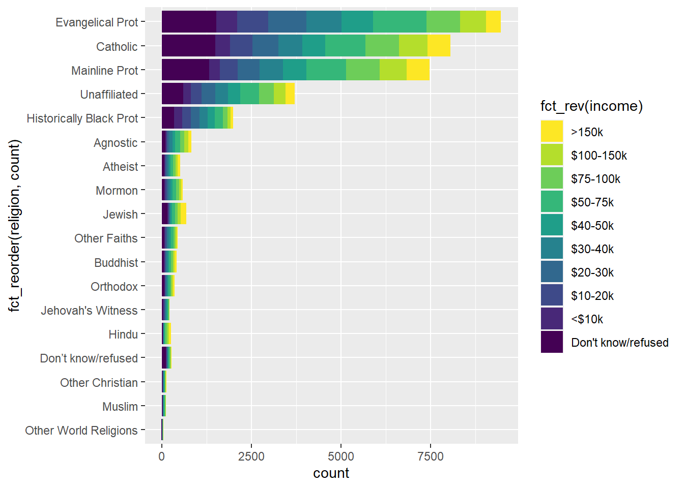 

Nonetheless, the un-pivoted, wide data, can be subset and visualized even though this is not ideal when attempting more complex visualization variations. Here, un-pivoted, I will make a bar chart of religious affiliation for incomes between $40k and $50k. Since I’m using just one variable, the code is not hard to compose. But note, the data re not in a tidy-data format.

relig_income %>% 
  ggplot(aes(fct_reorder(religion, `$40-50k`), `$40-50k`)) +
  geom_col() + 
  coord_flip()

Tidy, pivot_longer, data will be easier to manipulate with ggplot2. For example, You can subset the data with a single filter function, thereby more easily enabling different income charts. Below, the code is easier to read and easier to modify if I want to use a different income value.

filter(income == "$40-50k")

relig_income %>%
  pivot_longer(-religion, names_to = "income", values_to = "count") %>% 
  filter(income == "$40-50k") %>% 
  ggplot(aes(fct_reorder(religion, count), count)) +
  geom_col() +
  coord_flip()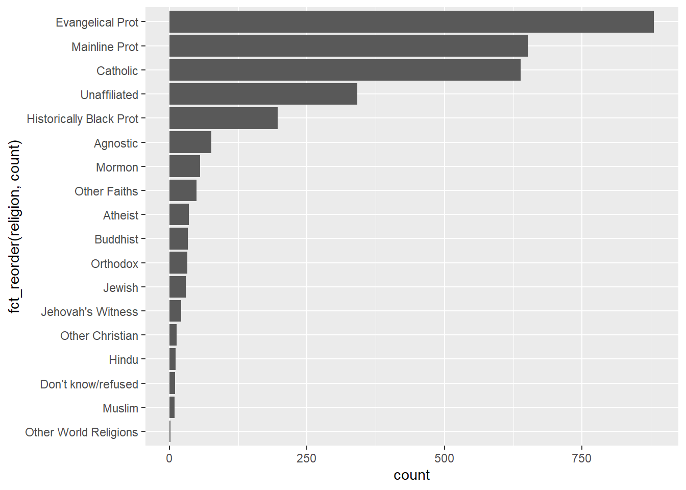 

Getting more complex, a natural step is to make comparisons across incomes. To do this we use ggplot2::facet_wrap()

relig_income %>%
  pivot_longer(-religion, names_to = "income", values_to = "count") %>% 
  mutate(income = fct_relevel(income, inc_levels)) %>% 
  ggplot(aes(fct_reorder(religion, count), 
             count)) +
  geom_col(show.legend = FALSE) +
  coord_flip() +
  facet_wrap(vars(income), nrow = 2)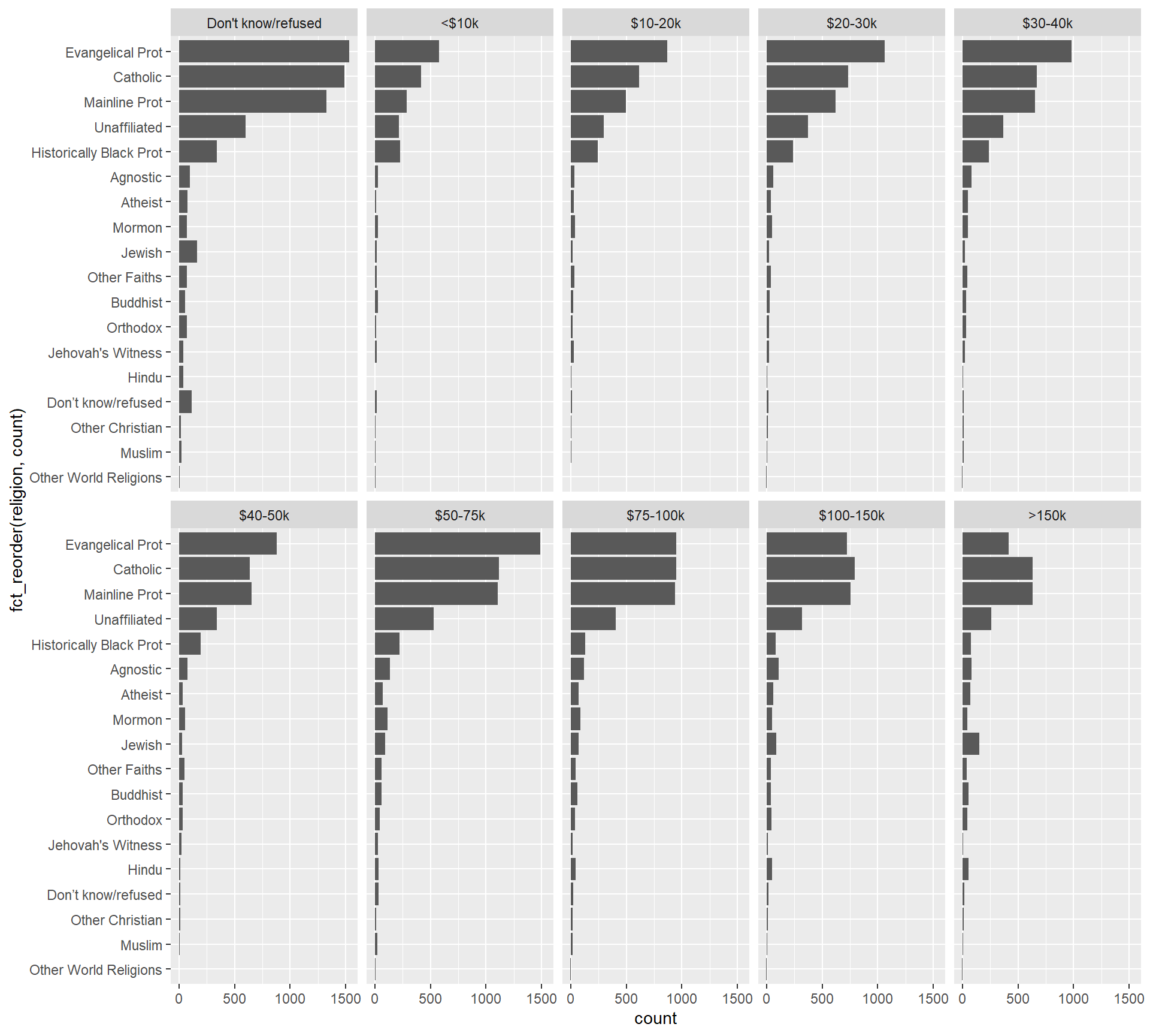

Another variation. Again, ggplot2 affordances are easier to leverage with tall data.

relig_income %>%
  pivot_longer(-religion, names_to = "income", values_to = "count") %>% 
  mutate(religion = fct_lump_n(religion, 4, w = count)) %>% 
  mutate(income = fct_relevel(income, inc_levels)) %>% 
  group_by(religion, income) %>%
  summarise(sumcount = sum(count)) %>% 
  ggplot(aes(fct_reorder(religion, sumcount), 
             sumcount)) + 
  geom_col(fill = "grey80", show.legend = FALSE) +
  geom_col(data = . %>% filter(income == "$40-50k"),
           fill = "firebrick") +
  geom_col(data = . %>% filter(income == ">150k"),
           fill = "forestgreen") +
  coord_flip() +
  facet_wrap(vars(income), nrow = 2)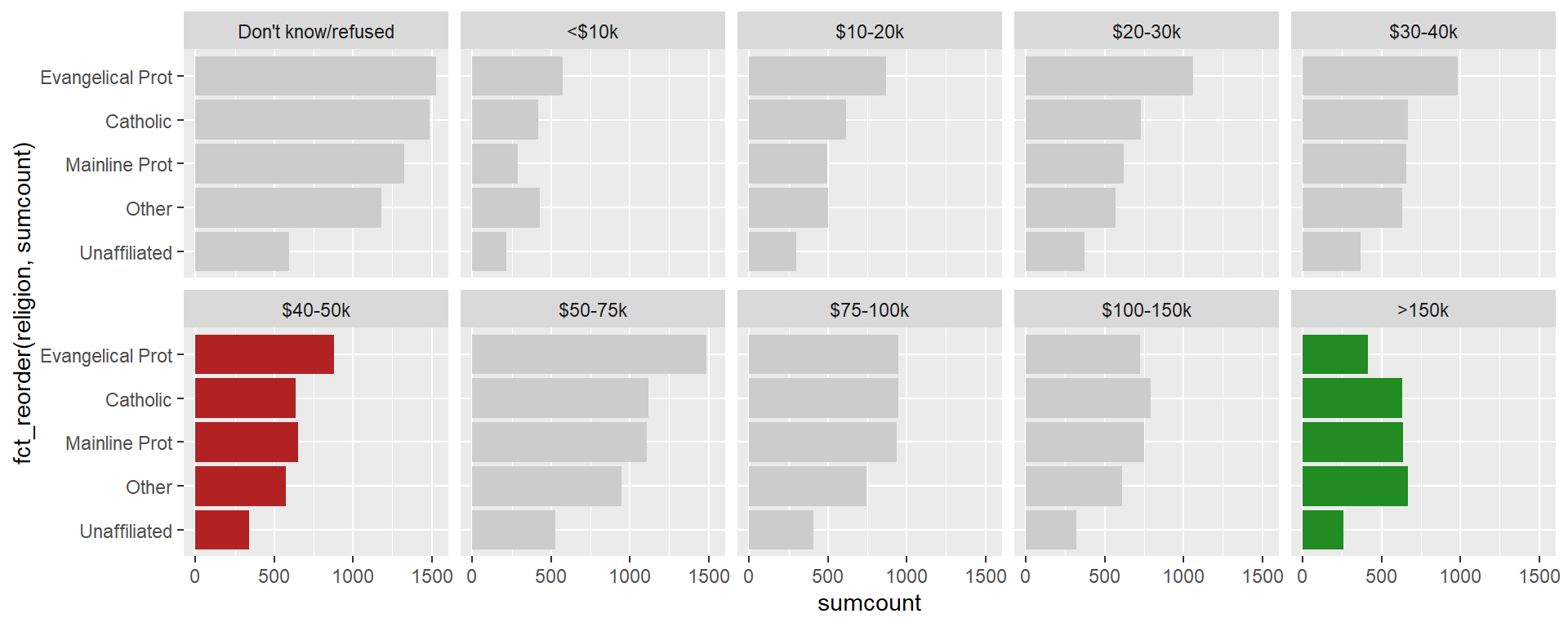 

References

Wickham, Hadley. 2014. “Tidy Data.” Journal of Statistical Software 59 (10). https://doi.org/10.18637/jss.v059.i10.

Wickham, Hadley, Mine Çetinkaya-Rundel, and Garrett Grolemund. 2023. R for data science : import, tidy, transform, visualize, and model data. 2nd edition. Sebastopol, CA: O’Reilly Media, Inc.

Footnotes

1. A robust discussion of tidy data can be found in R for Data Science (Wickham, Çetinkaya-Rundel, and Grolemund 2023): https://r4ds.had.co.nz/tidy-data.html